At some point, I think most statisticians have been asked about the difference between Bayesian and frequentist methods by a colleague outside of statistics. How do you answer that without scribbling conditional probability formulas on the nearest cocktail napkin? For a long time, I have wanted a strategy to motivate the difference for researchers who do not have any training in probability theory and thus, have never seen Bayes’ Rule.
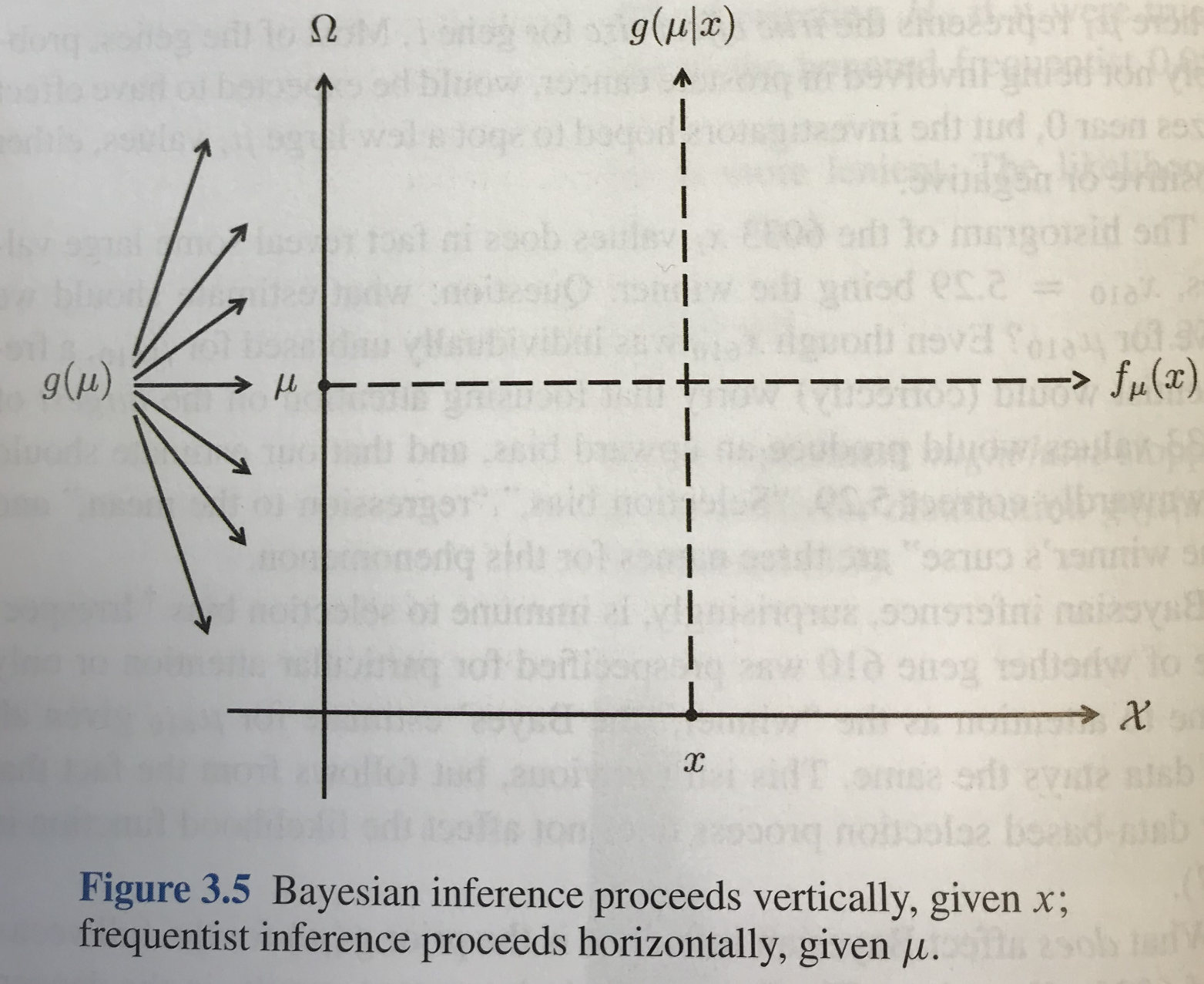
I recently encountered an interesting graphic in Computer Age Statistical Inference by Brad Efron and Trevor Hastie. Figure 3.5 in the book (included below) appears toward the end of the chapter on Bayesian Inference (after all of the usual probability formulas). The graphic is simple and lovely. The sample space is on the horizontal axis, the parameter space is on the vertical axis, the Bayesian approach proceeds vertically by considering the distribution of unknown parameters given observed data, and the frequentist approach proceeds horizontally by considering behavior of other data in the sample space for fixed (but unknown) parameters. Minimally, the graphic is a useful schema that summarizes the key distinctions between paradigms. I’ll be curious to determine whether this graphic might also be a useful diagram with which to introduce Bayesian methods to practitioners who have not taken a formal probability course and are already familiar with frequentist methods. I imagine using this figure to stimulate interest in Bayesian methods among non-statisticians in the future.
Efron, B., & Hastie, T. (2016). Computer Age Statistical Inference. Cambridge University Press.