Blog

People sometimes ask me how I got interested in statistics in the first place, expecting that I am either crazy or miserable. The truth is that my first experience with statistics was incredible. I finally wrote about my first statistics professor and hero Golde Holtzman for Amstat News, available here.

How My First Statistics Professor Changed My Life—A Tribute to Golde Holtzman

The title of this post is a quote from Smooth Jimmy Apollo, a fictional sports gambling prognosticator from “Lisa the Greek,” an episode of the Simpsons from season 3. The episode opens with Homer set for a couch-bound day of gluttony and illicit gambling on NFL games. During the pregame show, a television host introduces Jimmy, touting his 52% accuracy calling NFL games.  When pressed by the news host, Jimmy gives Denver the nod over new England, and Homer dutifully calls Moe’s Tavern with a $20 bet to that effect.  New England wins 55-10.  When asked about his bad prediction, Jimmy says, “Well folks, when you are right 52% of the time, you are wrong 48% of the time.” To which Homer responds “Why didn’t you say that before?”

Just under a week ago my childhood friend Chris Wilson called me to ask how I thought one might go about probabilistically predicting which Oscar nominee would win best picture in 2019 (award show this Sunday) based on the 381 films that have been nominated for the award between 1950 and 2018. CW is the director of data journalism at TIME.com, and he had just assembled a data set that includes 47 candidate predictors in the form of other awards and nominations for all historical nominees.

Unfortunately, the deadline to explain a modeling approach and furnish a prediction was about 4 days from our first discussion.

Under the time constraint posed, I suggested a simple off-the-shelf logistic regression approach with ad-hoc two-stage model selection to choose predictors. First, we ran a series of univariate logistic regressions and grabbed the top several contenders (chosen based on odds ratios), followed by an exhaustive model search in the top set using BIC as the selection metric. The modeling exercise (and a few variants) were fairly unequivocal that there is no lock, but, relative to the historical body of data, a film with Roma’s accolades was the best bet. You can check out the article here.

The exercise got me thinking about the various time scales on which statistical activity is of interest. For a methodological development to be published in a statistics journal, we expect to take months, devise optimal procedures to address novel problems, and fear the timeline will extend to years due to the extensive peer review process. (An analysis like ours would be desk-rejected by this sort of venue.) A responsible data analysis using best existing practices for a study outside of statistics likely takes weeks in my experience, and the total time to acceptance for publication is probably only months (although this varies widely by field). I have consulted with businesses and other groups to answer data-analytic questions for internal use, which sometimes takes only a few weeks.

But data journalism has a window of days. I have some specific ideas about how to exploit the unique structure of the Oscar prediction problem, and these will take time to develop. But the Oscars are imminent. Every day we postpone publishing drastically reduces the value of the article. Nobody cares if we correctly predict a past winner. And next week, the world (which moves more quickly than the publication cycle of statistics journals) will surely provide a new data challenge with a short timeline. So, without time to invent the perfect power trimmer for the task, we instead tended our data hedge with the logistic regression machete. Maybe I can get some better ideas together for the next award show. But for now, Godspeed, Roma. I have never cared more about the fate of a film that I have not yet had the chance to see.

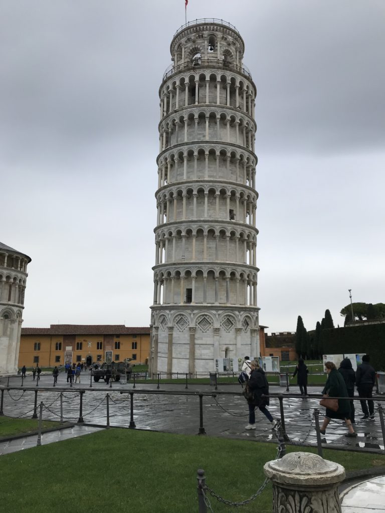
In December 2018 I attended CMStatistics for the first time at the University of Pisa in Italy. It was a great trip with the chance to meet new friends and eat a lot of pizza with my wife who joined me after the conference.

On a related note, here are some recent and upcoming talks

December 15, 2018, CMStatistics, University of Pisa, Italy. Objective Bayesian analysis for Gaussian hierarchical models with intrinsic conditional autoregressive priors

February 15, 2019, Conference on Statistical Practice, New Orleans, Louisiana. A practical assessment of the sensitivities of Bayesian model selection

April 1, 2019, James Madison University Department of Mathematics and Statistics. Assessing the sensitivities of p-values and Bayes factors.

April 2019, DATAWorks Defense and Aerospace Test and Analysis (DATA) Workshop, Springfield, VA. Categorical Data Analysis short course

May 2019, American Statistical Association/Institute of Mathematical Statistics Spring Research Conference, Blacksburg, Virginia. Detection of hidden additivity and inference under model uncertainty for unreplicated factorial studies via Bayesian model selection and averaging

May 2019, Association for Behavior Analysis International, Chicago, Illonois. The potential of statistical inference in behavior analysis: A panel with discussion

August 2019, International Conference on Statistics: Theory and Applications, Lisbon, Portugal. Assessing Bayes factor surfaces using interactive visualization and computer surrogate modeling

August 2019, Joint Statistical Meetings, Denver, Colorado. The primordial soup for Bayesian analysis in collaborative settings: technical skill, communication, and trust

In the least surprising development imaginable, I’m currently working on a manuscript that involves Bayesian model selection via Bayes factors. More details in the months to come, but one aspect of the project involves the extent to which Bayes factors are sensitive to prior specification. Within the context of Bayesian model selection, the researcher must specify two layers of prior belief. First, the researcher specifies priors on the space of candidate models. Second, priors are chosen for the parameters of those models. In a world simpler than ours, the prior on the model space would fully encapsulate known information and preferences among the candidate models. For example, setting the model prior to some flavor of a uniform distribution (on the models directly or perhaps a uniform distribution on classes of models of each size) would reflect an uninformed prior preference among the models.

As it turns out, the world is not so simple. Bayes factors are also sensitive (sometimes wildly) to the priors on the parameters. Generally, more diffuse priors on parameters lead to a preference for simpler models.  Further, the tail behavior of priors as related to likelihoods can have a surprising impact on resulting Bayes factors. For the purpose of fitting Bayesian models, usually an increase in the sample size lets the data (through the behavior of the likelihood function) increasingly dominate inference, so the choice of prior becomes less important. This is not so for Bayesian model selection, where increasing the sample size will often exacerbate problems due to the unfortunate choice of prior. Thus, two researchers who analyze the same data, choose the same likelihood function, select the same prior on the model space but use different priors on the parameters of the candidate models might get wildly different Bayes factors and hence conclusions, even when the differences in those priors might seem innocuous (e.g. do you prefer gamma(.1,.1)? gamma(.01,.01)? gamma(.0001,.0001)?). This instability is present in cases where Bayes factors can be calculated analytically. As a further difficulty, Bayes factors approximated via Monte Carlo Markov chain can be highly unstable, adding yet another layer of uncertainty into the metric which we are ostensibly using to gain certainty about which models are best supported by observed data.

I’ll confess that my initial interest in Bayes factors has been partially due to the fact that many arguments against p-values have merit. Bayes factors seem like a natural alternative to p-values for hypothesis testing and model selection. As a younger statistician, I even fantasized a bit about the possibility that Bayes factors might offer a panacea against certain drawbacks of p-values. Now I am not so sure. To those who rightly worry that hypothesis testing based on comparing p-values to specific thresholds is a process that is often “hacked,” it would seem that Bayes factors are much easier to hack.

So why continue my interest in Bayes factors? To me, there is something (beyond the obvious philosophical appeal) that is fascinating about Bayesian model selection based on Bayes factors. To use Bayes factors responsibly, you must explore their sensitivity to prior beliefs. This sensitivity analysis provides a formal way to understand where someone with a different worldview for their parameters might draw conclusions opposite to yours even when the observed data are agreed upon. I want science to move in a direction where researchers are rewarded less for increasingly sensational claims paired with a falsely overstated assertions of confidence. The idea that individual studies based on finite samples (often drawn for convenience) provide some inferential lens to the true state of the universe borders on hubris, come to think of it. So, for now, I hope Bayes factors will gain more traction because their analysis reveals such sensitivities. More to come.

As I write this it is 1:00 PM on Saint Patrick’s day in Blacksburg Virginia, four blocks from the Virginia Tech campus.  In a few hours I will leave my home to join a large gathering of undergraduate students.  You would be forgiven if you assumed we’d meet downtown to drink every green beer in sight. Instead, these students have traded the usual St. Paddy’s Day revelries to compete in DataFest, a 48 hour data analysis competition sponsored by the American Statistical association. An anonymous technology company partner has provided a 7 million row 42 column data set.  The analysis of these data forms the basis of the competition between undergraduate teams. My colleague and friend Christian Lucero organized the VT event. Faculty volunteers serve as “Expert Advisers,” which will be my role.  In addition to providing whatever potentially helpful guidance I can, I have some burning questions of my own for the students.

Namely, why have you chosen to engage in a weekend long St. Patrick’s Day-straddling data analysis competition that lies outside of your academic commitments and other responsibilities?

What does a competition like DataFest provide that motivates participation? Professors spend substantial effort trying to maximize classroom attendance and engagement. Is there something we can learn from DataFest that might help us create educational content that appeals to students? Will the DataFest participants articulate their motivations elegantly such that other students could be challenged to adopt similar views?

*****

I was not surprised to learn that the students who enrolled in the competition are highly motivated self-starters.  Students in the competition ranged from freshmen to seniors.  They gave a number of interesting answers to my question about their motivation. Virtually every student I spoke with described a desire to get “real” experience with big data.  Summarizing by academic level, this was articulated in distinct ways.  For instance, one freshman described a desire to “try out” data analytics to make sure they liked it before advancing too much further in their studies.  Upper class students described a desire to obtain experience that would be useful in the job market.  A number of students said they were enjoying the contest due to the realistic data setting, where a smaller set said they liked the group-oriented approach and fact that participation was not linked to a classroom grade. A similarly small set described a competitive motivation, wishing  to determine how well they “stack up” against their peers.

It was refreshing to spend time with students who are future-oriented and proactive to the extent that they spent the whole weekend analyzing data for experience and fun.  Can any of these observations be useful to motivate classroom behavior?  I don’t know.  I wish I could copy motivation from this highly driven set of students and paste it into the desires of all students. Perhaps the best strategy was one Christian Lucero used.  Her adjusted his class assignments and exams in such a way as to make participation in DataFest easier on the students.  Smart.  I think I will follow his lead by easing the course load in my classes around DataFest next year to encourage more students to participate.

At some point, I think most statisticians have been asked about the difference between Bayesian and frequentist methods by a colleague outside of statistics.  How do you answer that without scribbling conditional probability formulas on the nearest cocktail napkin? For a long time, I have wanted a strategy to motivate the difference for researchers who do not have any training in probability theory and thus, have never seen Bayes’ Rule.

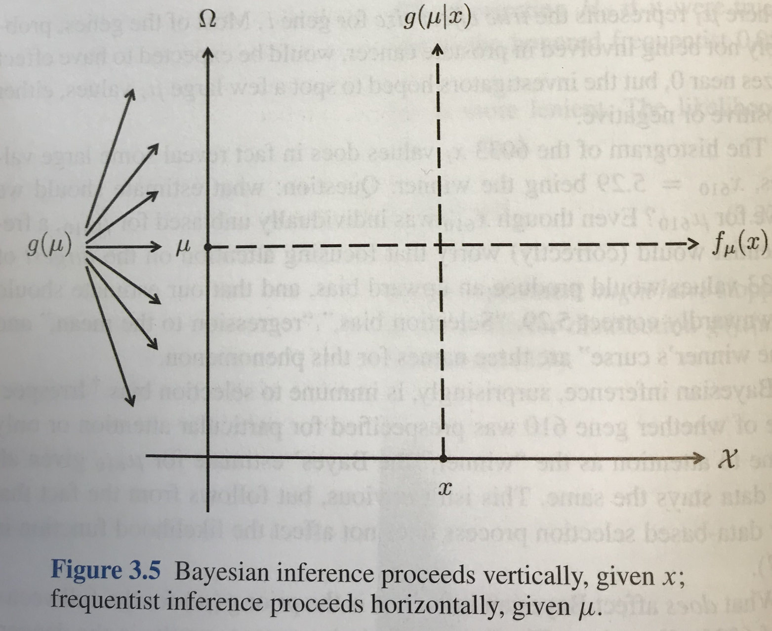
I recently encountered an interesting graphic in Computer Age Statistical Inference by Brad Efron and Trevor Hastie. Figure 3.5 in the book (included below) appears toward the end of the chapter on Bayesian Inference (after all of the usual probability formulas).  The graphic is simple and lovely. The sample space is on the horizontal axis, the parameter space is on the vertical axis, the Bayesian approach proceeds vertically by considering the distribution of unknown parameters given observed data, and the frequentist approach proceeds horizontally by considering behavior of other data in the sample space for fixed (but unknown) parameters. Minimally, the graphic is a useful schema that summarizes the key distinctions between paradigms.  I’ll be curious to determine whether this graphic might also be a useful diagram with which to introduce Bayesian methods to practitioners who have not taken a formal probability course and are already familiar with frequentist methods. I imagine using this figure to stimulate interest in Bayesian methods among non-statisticians in the future.

 

Efron, B., & Hastie, T. (2016). Computer Age Statistical Inference. Cambridge University Press.